如何快速實現REST API集成以優化業務流程
# 輸出

Using device: cuda此時會輸出運行環境是GPU還是CPU
? ? ? ?MNIST數據集是一個小數據集,存儲的是0-9手寫數字字體,每張圖片都28X28的灰度圖片,每個像素的取值范圍是[0,1],下面加載該數據集,并展示部分數據:
dataset = torchvision.datasets.MNIST(root="mnist/", train=True, download=True, transform=torchvision.transforms.ToTensor())

train_dataloader = DataLoader(dataset, batch_size=8, shuffle=True)

x, y = next(iter(train_dataloader))

print('Input shape:', x.shape)

print('Labels:', y)

plt.imshow(torchvision.utils.make_grid(x)[0], cmap='Greys');
# 輸出
Input shape: torch.Size([8, 1, 28, 28])
Labels: tensor([7, 8, 4, 2, 3, 6, 0, 2])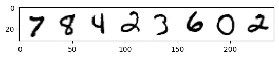
? ? ? ?所謂退化過程,其實就是對輸入數據加入噪聲的過程,由于MNIST數據集的像素范圍在[0,1],那么我們加入噪聲也需要保持在相同的范圍,這樣我們可以很容易的把輸入數據與噪聲進行混合,代碼如下:
def corrupt(x, amount):

  """Corrupt the input x by mixing it with noise according to amount"""
  noise = torch.rand_like(x)
  amount = amount.view(-1, 1, 1, 1) # Sort shape so broadcasting works
  return x*(1-amount) + noise*amount
接下來,我們看一下逐步加噪的效果,代碼如下:
# Plotting the input data

fig, axs = plt.subplots(2, 1, figsize=(12, 5))

axs[0].set_title('Input data')

axs[0].imshow(torchvision.utils.make_grid(x)[0], cmap='Greys')


# Adding noise

amount = torch.linspace(0, 1, x.shape[0]) # Left to right -> more corruption

noised_x = corrupt(x, amount)


# Plottinf the noised version

axs[1].set_title('Corrupted data (-- amount increases -->)')

axs[1].imshow(torchvision.utils.make_grid(noised_x)[0], cmap='Greys');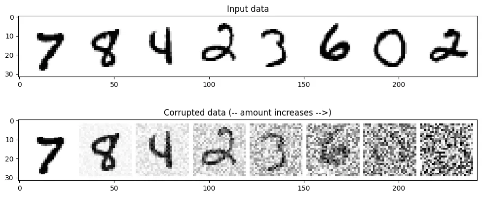
從上圖可以看出,從左到右加入的噪聲逐步增多,當噪聲量接近1時,數據看起來像純粹的隨機噪聲。
? ? ? ?UNet模型與自編碼器有異曲同工之妙,UNet最初是用于完成醫學圖像中分割任務的,網絡結構如下所示:
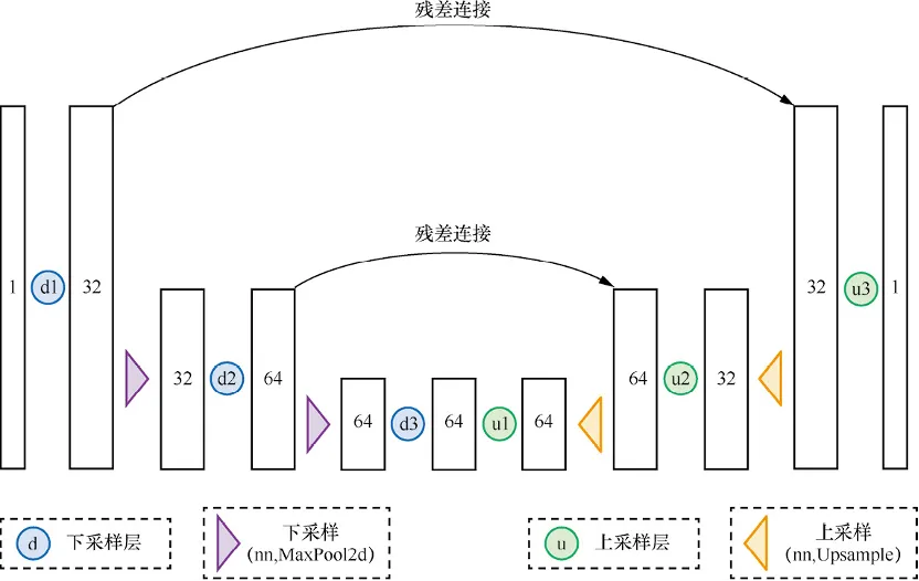
代碼如下:
class BasicUNet(nn.Module):

    """A minimal UNet implementation."""

    def __init__(self, in_channels=1, out_channels=1):

        super().__init__()

        self.down_layers = torch.nn.ModuleList([

            nn.Conv2d(in_channels, 32, kernel_size=5, padding=2),

            nn.Conv2d(32, 64, kernel_size=5, padding=2),

            nn.Conv2d(64, 64, kernel_size=5, padding=2),

        ])

        self.up_layers = torch.nn.ModuleList([

            nn.Conv2d(64, 64, kernel_size=5, padding=2),

            nn.Conv2d(64, 32, kernel_size=5, padding=2),

            nn.Conv2d(32, out_channels, kernel_size=5, padding=2),

        ])

        self.act = nn.SiLU() # The activation function

        self.downscale = nn.MaxPool2d(2)

        self.upscale = nn.Upsample(scale_factor=2)


    def forward(self, x):

        h = []

        for i, l in enumerate(self.down_layers):

            x = self.act(l(x)) # Through the layer and the activation function

            if i < 2: # For all but the third (final) down layer:

              h.append(x) # Storing output for skip connection

              x = self.downscale(x) # Downscale ready for the next layer


        for i, l in enumerate(self.up_layers):

            if i > 0: # For all except the first up layer

              x = self.upscale(x) # Upscale

              x += h.pop() # Fetching stored output (skip connection)

            x = self.act(l(x)) # Through the layer and the activation function


        return x
我們來檢驗一下模型輸入輸出的shape變化是否符合預期,代碼如下:
net = BasicUNet()

x = torch.rand(8, 1, 28, 28)

net(x).shape
# 輸出
torch.Size([8, 1, 28, 28])再來看一下模型的參數量,代碼如下:
sum([p.numel() for p in net.parameters()])# 輸出
309057至此,已經完成數據加載和UNet模型構建,當然UNet模型的結構可以有不同的設計。
? ? ? ?擴散模型應該學習什么?其實有很多不同的目標,比如學習噪聲,我們先以一個簡單的例子開始,輸入數據為帶噪聲的MNIST數據,擴散模型應該輸出對應的最佳數字預測,因此學習的目標是預測值與真實值的MSE,訓練代碼如下:
# Dataloader (you can mess with batch size)
batch_size = 128
train_dataloader = DataLoader(dataset, batch_size=batch_size, shuffle=True)
# How many runs through the data should we do?
n_epochs = 3
# Create the network
net = BasicUNet()
net.to(device)
# Our loss finction
loss_fn = nn.MSELoss()
# The optimizer
opt = torch.optim.Adam(net.parameters(), lr=1e-3)
# Keeping a record of the losses for later viewing
losses = []
# The training loop
for epoch in range(n_epochs):
for x, y in train_dataloader:
# Get some data and prepare the corrupted version
x = x.to(device) # Data on the GPU
noise_amount = torch.rand(x.shape[0]).to(device) # Pick random noise amounts
noisy_x = corrupt(x, noise_amount) # Create our noisy x
# Get the model prediction
pred = net(noisy_x)
# Calculate the loss
loss = loss_fn(pred, x) # How close is the output to the true 'clean' x?
# Backprop and update the params:
opt.zero_grad()
loss.backward()
opt.step()
# Store the loss for later
losses.append(loss.item())
# Print our the average of the loss values for this epoch:
avg_loss = sum(losses[-len(train_dataloader):])/len(train_dataloader)
print(f'Finished epoch {epoch}. Average loss for this epoch: {avg_loss:05f}')
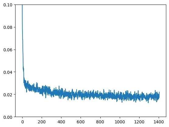
# View the loss curve
plt.plot(losses)
plt.ylim(0, 0.1);# 輸出
Finished epoch 0. Average loss for this epoch: 0.024689
Finished epoch 1. Average loss for this epoch: 0.019226
Finished epoch 2. Average loss for this epoch: 0.017939訓練過程的loss曲線如下圖所示:
我們選取一部分數據來評估一下模型的預測效果,代碼如下:
#@markdown Visualizing model predictions on noisy inputs:


# Fetch some data

x, y = next(iter(train_dataloader))

x = x[:8] # Only using the first 8 for easy plotting


# Corrupt with a range of amounts

amount = torch.linspace(0, 1, x.shape[0]) # Left to right -> more corruption

noised_x = corrupt(x, amount)


# Get the model predictions

with torch.no_grad():

  preds = net(noised_x.to(device)).detach().cpu()


# Plot

fig, axs = plt.subplots(3, 1, figsize=(12, 7))

axs[0].set_title('Input data')

axs[0].imshow(torchvision.utils.make_grid(x)[0].clip(0, 1), cmap='Greys')

axs[1].set_title('Corrupted data')

axs[1].imshow(torchvision.utils.make_grid(noised_x)[0].clip(0, 1), cmap='Greys')

axs[2].set_title('Network Predictions')

axs[2].imshow(torchvision.utils.make_grid(preds)[0].clip(0, 1), cmap='Greys');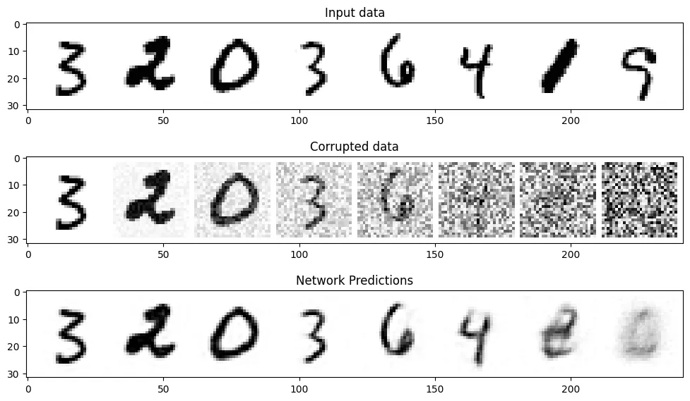
從上圖可以看出,對于噪聲量較低的輸入,模型的預測效果是很不錯的,當amount=1時,模型的輸出接近整個數據集的均值,這正是擴散模型的工作原理。
Note:我們的訓練并不太充分,讀者可以嘗試不同的超參數來優化模型。
文章轉自微信公眾號@ArronAI